Meet Udeshi

Everybody has this presumed notion that noise in an electronic system is bad. We all learn about ways to reduce noise in the circuits we implement to get better results. In this post we will see a case where intentionally adding noise to a system will give better results.

What is wrong with a normal ADC?

The purpose of an Analog to Digital converter is to obtain a digital value of an analog signal. Lets say we want to convert a signal which is between -1 to 1V. The analog version of this signal will be a real number and so can take one of infinitely many real values between -1 and 1. But the digital representation will only be able to take finite number of values because we only have a finite number of bits to encode the real number.

We will have to quantize the signal i.e. pick the closest possible approximation of it from the set of possible values. For the sake of simplicity, lets assume we have just 1 bit to encode the signal. So the set of values our digital signal can take is \(\{0, 1\}\). Now it is clear that depending on the analog value we will have to pick one of 0 or 1 to represent this value as our digital signal. The analog signal will almost never equal to -1 or 1 (try calculating the probability) so we will always get an error when we try to quantize our signal. This error is called Quantization Error.

There is already an error and you want to add more noise?!

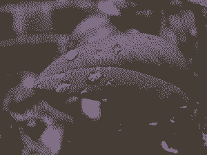
We will eventually see that intentionally adding noise will help reduce quantization error. This kind of intentionally added noise is so commonly used that it has its own name: Dither. Dither, apart from being used in ADCs is very widely used in image processing to display better quality images. See an example from the wikipedia page:

The image of this leaf has been represented using just the colour white(1) and black(0)! And yet it looks like it has various shades of grey! Lets see how this happens.

Dither in ADCs

Continuing with the quantization example above, lets say we have a 1-bit ADC which gives output 0 if the input signal is negative and 1 if positive. If \(X\) is the digital output and \(c\) is the analog input (assumed constant),

If we add a dither \(d(t)\) to the analog input, the value of \(X\) will be decided by \(c+d(t)\). Lets say we add a dither which is characterised by a uniform random variable, so

we will later see the significance of the range \(-\frac{1}{2},\frac{1}{2}\). Cumulative density function of \(d\) will be

\(X\) is dependent on a random variable, hence \(X\) will also become a random variable. And because \(X \in \{0,1\}\) it will be a Bernoulli random variable

Hence,

We get \(X\) to be a be a bernoulli variable with parameter dependent on our analog value!

We can see that expected value of \(X\) is equal to \(c + \frac{1}{2}\) (because X is bernoulli). By the law of large numbers, we can say that if we take large number of samples of \(X\) (keeping \(c\) constant), the average value of these samples will converge to the expected value \(c + \frac{1}{2}\)

Block diagram for adding dither

The Sampler just reads the value of its input at \(t = nT\), hence it gives a sample at every \(T\) seconds. From our previous derivation we can say that

The problem here is that taking an infinite number of samples will take infinite time which is impractical. But we can say that the larger number of samples we the better accuracy in value of \(c\) we will get. If we take \(n\) samples, we can see that the average of \(X[n]\) will take one of \(n\) values from the set \(\{0,\frac{1}{n},\frac{2}{n},...,\frac{n}{n}\}\).

We thus have quantized \(c\) to \(n\) distinct values or \(\text{log}_2(n)\) bits using a 1-bit ADC!

Dither in images

Lets take a look at the leaf image once again. Observe that a greyscale image has been approximated here using two distinct values (black and white) i.e. a 1-bit value. Such an image is called a binary image.

Lets say the greyscale had values for every pixel as a real number between 0 and 1, 0 corresponding to full black and 1 corresponding to full white. There would be regions in this image with similar values of grey. For e.g. take the section of the top of the leaf. It is a region of light grey (value\(=c>\frac{1}{2}\)). If we convert this region directly to binary, the whole region will become white. Similarly we would get a large patches of black and white all over the image which would be a pretty inaccurate depiction of the greyscale image.

Now if we add dither to that small region of similar greyscale value and then convert to binary image, the probability of getting a white pixel will be proportional to the value of that region (\(=c\)). If the region has 100 pixels, instead of all 100 being converted to white pixels, \(100c\) pixels will be white and \(100(1-c)\) will be black. On average that will look like the region is grey with value \(c\).

We can say that the average value of a small region in the binary image will be close to the greyscale value of that small region in the real image. Hence we can see that dither gives us a better approximation after quantization.

Note: The leaf image is using a slightly better algorithm than just adding dither and converting to binary (Random dithering). Such an image would look much worse, so for representative purposes I have used this image. You can read more about better algorithms on the wikipedia page of Dither